MULTI-BODY SOLVER
The Multi-Body Dynamic (MBD) solver is a general purpose tool capable of simulating any mechanical system. The basic assumptions of MBD are that bodies under consideration are rigid, and all joints are frictionless. The number of bodies and joints is arbitrary, and thus total number of Degrees of Freedom (DoFs) is arbitrary. It is up to the user to decide how complex a system should be.
There are two versions of the code. The MATLAB proof of concept version is available under MIT License on GitHub - https://github.com/windflow-pl/MBDM. The other, C version of the code or its source, can be requested using contact form.
Example of a wind turbine model in MBD.
Kinematic analysis of a wind turbine model in MBD.
Concept and essential formulation
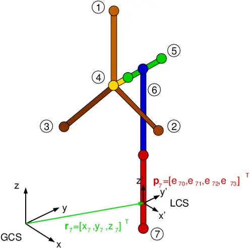
Each body is assigned a local coordinate system, which is attached to the body and follows its translational and rotational motions. The position and orientation of each body is then described in the global coordinate system by seven quantities: vector r = [x,y,z]T pointing to the local coordinate system of the body, and the Euler parameters p = [e0,e1,e2,e3]T ≡ [e0,e]T indicating orientation of body frame in global coordinate system.
Any given vector in the body coordinate system can be transferred to the global coordinate system vector using transformation matrix A, which is given as
| e02 + e12−1/2 | e1e2 − e0e3 | e1e3 + e0e2 |
| e1e2 + e0e3 | e02 + e22 − 1/2 | e2e3 − e0e1 |
| e1e3 − e0e2 | e2e3 + e0e1 | e02 + e32 − 1/2 |
Matrix A and is a rotational matrix, which becomes identity matrix if both frames coincide. Therefore, if point P is described by vector s′P in body local reference frame, the location of this point rP in global coordinate frame can be found by the following expression: rP = r + As′P where r = [x,y,z]T is the vector pointing to the location of body local coordinate system.
Constraints equations
System of constrained equations Φ(q,t) should ba assembled in order to begin with a problem. There are four basic constraints that relate two vectors or points defined in two different coordinate frames. Here we will give only a brief example, and full documentation can be referenced for detailed derivation.
Lets derive a constraint of orthogonality of two body-fixed vectors ai and aj on bodies i and j, respectively. Two vectors are orthogonal if their scalar product is zero: Φd1(ai,aj) ≡ aiTaj = 0 where the superscript notation d1 indicated the first form of dot product condition. Writing the vectors ai and aj in terms of their respective body reference frames using transformation matrices, ai = Aiai′ and aj = Ajaj′, the final constraint equation can be derived as Φd1(ai,aj) = ai′TAiTAjaj′ = 0
Kinematic analysis of a Quick Return mechanism in MBD.
Kinematic analysis
Each body i is assigned a generalised coordinate vector in a system qi = [ri,pi]T. The composite set of generalised coordinates for the entire system of all bodies is thus q = [q1T,q2T,...,qnbT]T where nb is the number of all bodies in the system. The combined system of kinematic, driving, and Euler parameter normalisation constraint equations that determines the position and orientation of the system is
| Φ1(q,t) |
| Φ2(q,t) |
| ... |
| Φnc(q,t) |
where nc is the number of all constraint equations defining the system.
The kinematic constraint equations are highly nonlinear. Therefore, the iterative Newton-Raphson technique is adopted to solve set of constraint equations. The Jacobian matrix of the constraint equations must be calculated to this end.
| Φx11 | Φy11 | ... | Φenb1 |
| Φx12 | Φy12 | ... | Φenb2 |
| ⋮ | ⋮ | ... | ⋮ |
| Φx1nc | Φy1nc | ... | Φenbnc |
The Newton-Raphson scheme can be summarized as follows qi + 1 = qi − Φ(qi,t)/Φq where q0 is the initial estimate of the assembled configuration and improved estimates are obtained by solving the sequence of equations. If the kinematic, driving and Euler parameter normalisation constraints are independent and if all degrees of freedom are constrained, the Jacobian is nonsingular. Thus, there is a unique solution for the position and orientation of the system.
Once position is computed, velocities and accelerations can be obtained by chain rule differentiation.
Dynamic analysis
Derivation of dynamic equations is far more lengthy, and it is not covered in this article. The MDBM documentation can be consulted for details. The resulting Euler parameter system of acceleration equations is obtained as:
| M | 0 | ΦrT | 0 |
| 0 | 4GTJ′G | ΦpT | ΦppT |
| Φr | Φp | 0 | 0 |
| 0 | Φp | 0 | 0 |
| r″ |
| p″ |
| λ |
| λp |
| FA |
| 2GTn′A + 8ĠTJ′Ġp |
| γ |
| γp |
Once solved for accelerations, then velocities and positions of independent variables can be obtained by integration. And dependent variables can be computed from kinematic analysis with independent variables already known. MBD performs automatic dependent/independent variables assignment on every time step for better stability.
Validation
Multiple tests were carried to validate the MBD implementation. Some relatively simple mechanism have readily available benchmark data.
The MBD was successfully tested against:
- two-dimensional slider-crank mechanism with known kinematic and dynamic solutions;
- three-dimensional slider-crank mechanism with known kinematic solution;
- gyroscopic mechanism with known analytical solution.
As an example, consider a tree-dimensional slider-crank mechanism shown below. The revolute joint is used to connect the crank (body 1) to the ground body, where the ground constraint is placed on body 4. The spherical joint is used to connect the crank to the rod (body 2), and then the revolute-cylindrical joint is used to connect the rod to the slider (body 3). The translational joint between the slider and the ground is placed to permit only one direction of motion for the slider. Finally, the distance constraint between the rod and the slider is employed to prevent the rod from sliding inside the slider. The revolute driver is imposed on the crank, with a constant rotational velocity of −2π. The notation is indicated in figure below. The resulting system has 4·6 = 24 degrees of freedom restricted by 5+3+3+5+1+6+1 = 24 independent equations.
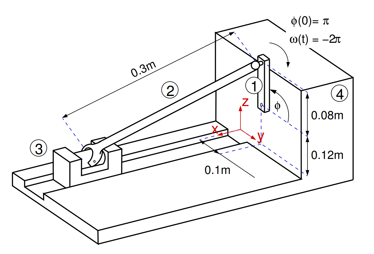
Example of a 3D slider crank mechanism.
Kinematic analysis of a 3D slider crank mechanism in MBD.
At time t=0, the crank was placed at angle π relative to the global y axis. The results of kinematic analysis are presented below, where the solution of the MBD solver is compared to the solution obtained by [1]. Good agreement can be seen.
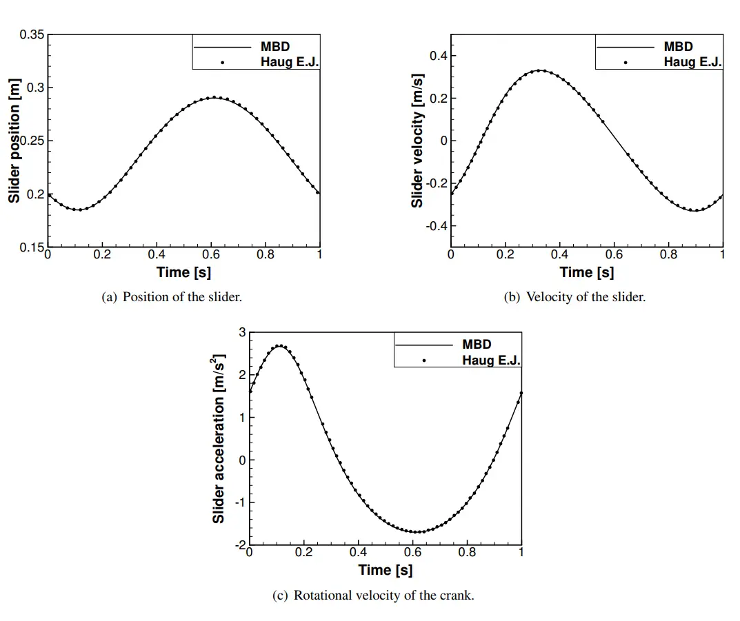
Comparison of results obtained with MBD and by [1].
Another example is a gyroscopic wheel that was used to validate that the gyroscopic effect is properly accounted for in the multi-body formulation. The model involves three bodies, as shown below. The ground body was placed at the origin at the global coordinate system. A short rod of length 0.1m was attached to the ground body at height 1.0m using an universal joint such that rotation along the rod axis is constrained. The other end of the rod was connected to the centre of mass of the steel wheel with a revolute joint. A constant rotational speed of 60rad/s was applied to the wheel by a revolute driver. The system has overall 2 unconstrained degrees of freedom - rotation about the direction of global axes z and y. The gravitational force acting in the negative z direction was applied to all bodies, and at time t = 0 the system was assumed to have no precession.
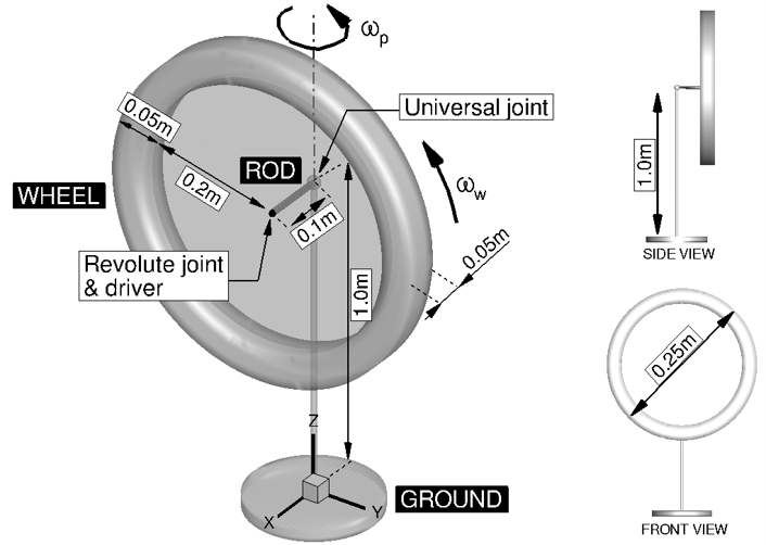
Schematic of the MBD gyroscopic simulation set-up.
The result of the dynamic computation is presented below, where the Runge-Kutta integration scheme of fourth order was employed, with a time step ∆t = 0.001s. As can be seen, the rate of precession developed in less then 0.1s, and then maintained almost constant value that agreed with the one obtained using the gyroscopic approximation.
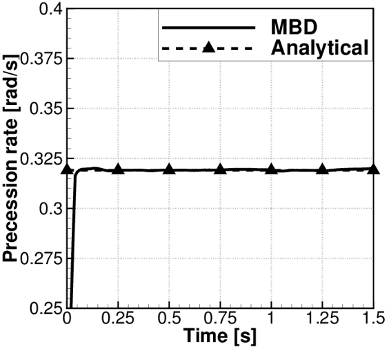
Obtained results of gyroscopic simulation with MBD.
Final words
Feel free to explore the code at https://github.com/windflow-pl/MBDM. We have prepared some examples to get you started. You may request more information using contact form.
[1] Haug E.J, Computer Aided Kinematics and Dynamics of Mechanical Systems. Vol. 1: Basic Methods, Allyn & Bacon, Inc., 1989